FPGA Drum Simulation

GitHub Link

fpga_drum repo

Introduction

Back in the fall of 2019 I took MIT’s FPGA-centric digital design lab (6.111) and was fortunate enough to have taken the course with a couple friends who were my teammates on our final project. One of my teammates was a percussionist in MITSO who was quite interested in making an electronic drum pad for the final project, so that’s what we settled on. I was not a percussionist, but I had what I thought to be a pretty creative--if not out-there--idea to synthesize the drum sounds. Rather than use an IFFT or FIR filter or base the output on any data recorded from a physical drum, I figured we could simulate the drum membrane in real-time and generate audio from that.

It might sound a little over-the-top, but I didn’t think of that on the spot. I had done a couple side projects in the years prior that convinced me the idea was actually more feasible than it might sound.

I had a bit of an obsession with using coupled-oscillator simulations to generate colorful wave-like patterns for LED displays of various kinds. The first was a sound activated lamp that used a 1D coupled-oscillator simulation mapped to a color gradient to make a cool sound-to-light display. I was so pleased with the 1D version that I decided to extend it to 2D on a 40x100 LED display. The idea there was to get the display to look like the surface of water, but I eventually realized the 2D coupled oscillator neglected many effects that are present in waves on the surface of liquids, and more than anything else was a good model of waves in a thin piece of solid material. Plus, my hall mates all agreed that basic animations looked a lot better than the wave simulation, which just looked like noise to the casual observer.

When we started working on the drum project, I realized the coupled oscillator simulation was perfect. What is a drum membrane other than a thin piece of solid material with waves travelling through it? Moreover, I knew from the LED display that a processor with a floating point unit running with a 250MHz clock could solve a time step for a 40x100 mass coupled oscillator about 20 times per second. Typical audio runs at something like 20-48 ksps, so that’s just…a 1000x speed boost that would be required. It would certainly be ambitious, but it sounded like the perfect project for an FPGA!

That semester, while my teammates focused on the analog front end for the drum pad and a graphical display to visualize the simulated drum membrane, I toiled away at implementing the coupled oscillator simulation in SystemVerilog. That semester we got a basic version working using fixed-point arithmetic, but we never really got it sounding all that good by the time the semester came to a close. I was really scratching my head, and the only explanation I could think of was that round off error was accumulating and throwing off the simulation, but it was too late to change the implementation to use floating point instead.

When the 6.111 professor announced there would be a special subject that J-term to continue working on FPGA projects, I was itching to give this project another go with floating-points. Plus, I had been having such a good time working with my teammates that I couldn’t pass up the opportunity to keep working with them. Thus began the project described below in January 2020.

The Simulation Model

First, it would probably be good to review the math behind the coupled oscillator model in case you aren’t familiar. I won’t go into too much detail since there are plenty of other sources that go into far more detail than I could, but I’ll run down the basics.

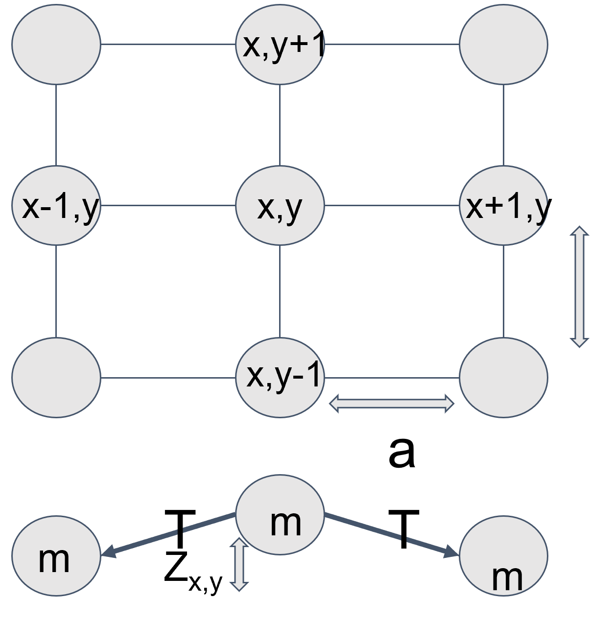
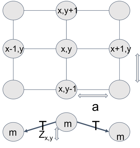
Imagine you have a grid of mass M all separated from each other with equal spacing a (ignore units for now). Now imagine all of these masses are connected to their nearest neighbors (i.e. the 4 masses in front of, behind, to the left, and to the right) with strings that have a tension T. I’ve included a diagram below to help visualize.

Now, imagine pulling one of the masses out of the page (i.e. applying a force perpendicular to the plane of the grid). You would feel a restoring force from the tension in the strings pulling the mass back downwards. Furthermore, the neighboring masses would experience a force pulling them out of the page via the strings, as would their neighbors, and their neighbors, etc. If you were then to let go of the mass, it would get pulled back to its original position and then overshoot it and begin oscillating, applying force to its neighbors in the process, causing them to oscillate too. The system would continue oscillating forever if there wasn't a damping force acting on each mass, which is generally represented by a force that’s inversely proportional to each mass’s velocity.

The cool thing about the system described above is that it’s really easy to figure out the force balance on each mass at any given time based on its velocity, its position, the positions of its neighbors, and any outside forces being applied to it. Using Newton’s second law, you can to define the equations of motion for each mass in the system, which allows you to calculate how the positions and velocities of each mass will change over time.

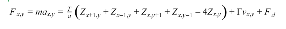
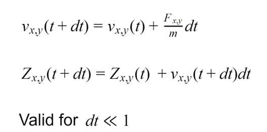
In this case, we solve the equations of motion numerically using the Euler-Cromer method, as regular Forward Euler is unstable and will eventually diverge. This essentially involves breaking time into small discrete steps, which allows you to approximate the change in each mass’s position as a linear function of its velocity and the change in each mass's velocity as a linear function of its acceleration. This essentially converts this system of differential equations into a series of arithmetic operations that are easy for a computer or FPGA to calculate.

Now, the system we just described might not really sound like a drum, but imagine adding more and more masses to the system while at the same time making them lighter and lighter and closer and closer together. At a certain point, it would be impossible to tell the difference between the grid of discrete masses and a continuous sheet of mass. A continuous sheet of mass is not so different from a drum membrane. The one additional nuance is that on a drum, the edges of the sheet are held in place by the drum body and don’t move. In our model above, that is equivalent to treating the masses along the edge as if one (or two on the corners) of its neighbors always has a constant position. This is known as a fixed boundary condition.

So now that we have a mathematical representation that reasonably approximates the motion of a drum membrane, how do you generate audio from it? I just assumed you could treat the drum sort of like a speaker cone, where the audio signal is roughly proportional to the average position of all the masses. Thus, simply summing the positions of all the masses in the system will give you your audio signal. I'll admit this isn't the most scientific approach, as in reality the drum membrane interacts with the surrounding air to create pressure waves, which would be much more difficult to model. Nevertheless, the "speaker" approach produced reasonable enough results.

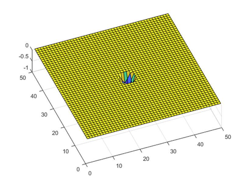
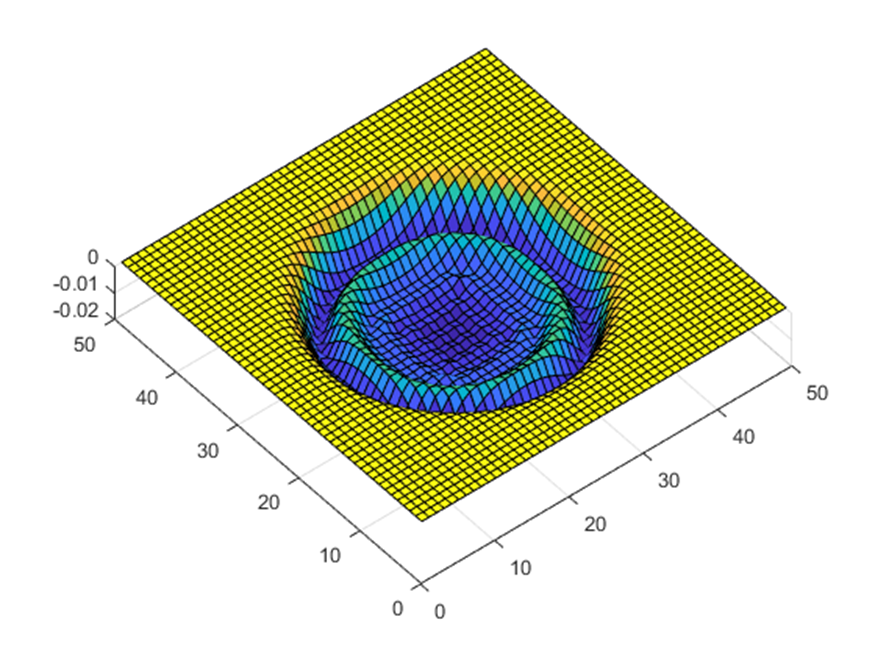
To confirm that this sort of system would actually sound like a drum, I wrote a Matlab script to simulate a 50x50 mass system and produce a 1 second long 48 ksps audio clip. Rendering that clip took about 2 hours, though Matlab is not generally known for its speed.

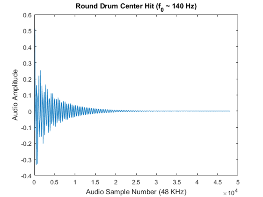
It might sound kind of crazy to generate drum sounds this way, but hear me out. For one thing, drum sounds actually have a fairly rich harmonic structure that is not trivial to replicate. That’s why a lot of synthesized drum sounds you hear in EDM don’t actually sound very realistic (at least to my ears). Even a relatively small coupled oscillator simulation produces many harmonics without having to mess around with FFTs or anything too complicated. Plus, there are actually a lot of nuances to the quality of sound a drum makes based on where you hit it (i.e. hitting a drum on the edge sounds different from hitting it dead center). This behavior would be a fair bit of work to replicate in a more conventional way, but it falls out of the simulation completely naturally without any extra effort. Finally, it’s pretty easy to change parameters of the simulation, such as tension and damping to impact the sound, much like how you can tune a timpani and dampen it after a hit.

You get all of these features for free simply by continuously generating an audio signal from the simulation described and using the input from a position and force-sensitive drum pad to apply a driving force to a mass in the appropriate position (though dynamically changing the damping and tension would require a couple extra bells and whistles for inputs). Of course, the difficulty comes in getting such a simulation to run fast enough to generate audio in real time. That’s where a custom hardware processing pipeline implemented in an FPGA becomes necessary.

The Basic Architecture

For this iteration of the project, I decided to use floating points for the simulation. The initial iteration used fixed point, but I was convinced that round-off error was causing the simulation to misbehave. In the end, it turned out that the Forward Euler method I had originally implemented to solve the equations of motion is problematic. Of course, I didn’t realize that until I had already completed a floating point implementation, which had the exact same problems as the fixed point version. Switching over to the Euler-Cromer method solved all the problems immediately. Nevertheless, all position and velocity values used in the simulation were represented by 32-bit single-precision floating points. In retrospect, using fixed point would have been faster, saved a lot of headaches, and could have freed up a lot of resources to run a larger simulation. Now I know for the future, I suppose.

Now the real pain of using floating points is that you can’t simply type out arithmetic operations and expect them to work. Fixed-point multiplication still requires some additional handling beyond simply placing a * between two operands, but not nearly as much as floating point. Luckily, Xilinx provides plenty of floating-point IP modules, so I didn’t need to worry about the nitty gritty of performing the arithmetic. All I had to do was figure out how to wire up a bunch of these IPs to to create a floating-point processing pipeline that would perform all the operations described above for the timestep of each mass. I’ll go more into detail on that component below, but for now just think of it as a black box where input position and velocity values for the current timestep are streamed in and position and velocity values for the next time step are streamed out.

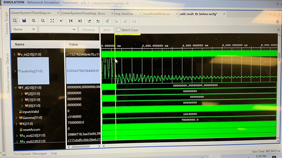
I built out the floating point pipeline by first focusing on a single mass system, then extending it to a small 1D system, and then finally a small 3x3 2D system. This allowed me to more easily verify that my code was working by looking at how the position values evolved in a testbench using the waveform viewer in Vivado.

Once I had a small 2D system working, it was time to scale it up to something larger. At that point it became clear that we couldn’t simply store all the simulation data as registers, so I had to figure out a way to write and read values into BRAM without adding too much latency. This is another place where the flexibility of FPGA hardware really shines. Generally, memory is organized into small data words (e.g. 8 or 16 bits) accessed using a large number of address, however taking that approach would have required hardware to perform tons of read operations for every time step of the simulation. This would have added an acceptable amount of overhead to each simulation time step. However, an FPGA provides the flexibility to generate BRAM with data words that are thousands of bits wide. Using a scheme like that, we could access data for a much larger number of masses in the same read operation, greatly reducing overhead.

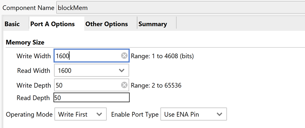
The physical system described above gave a pretty good insight into how the memory should be organized. If you think back to the grid of masses in the system and look a bit closer at the equations of motion, you can see that in order to solve the next time step for any column of masses all you need are the positions and velocities of that column as well as the positions of its two (or one in the case of the edges) neighboring columns. Thus, it’s fairly intuitive to simply store all the position values for an entire column in a single address location in BRAM. The same could be done for the velocities, which would be stored in a separate BRAM allowing it to be read at the same time as the position BRAM. We were targeting a 50x50 mass system, so that would require a bit width of 50*32=1600 bits. The maximum bit width allowed for BRAM on the Artix7 is 4608, so this scheme is totally feasible, though you obviously couldn’t scale it arbitrarily.

Once read out from the BRAM, the positions and velocities for each mass can be cached in a register array, where the index of the array specifies the row index in the grid of masses, and the address read from BRAM represents the column index. To store the inputs, we would need four such register arrays, two for the positions and velocities of the column we are calculating for, and two for the positions of its two neighboring columns. We would also need an additional two register arrays to store the output positions and velocities for the column we are calculating. That’s still a lot of registers, but far fewer than would be required by the entire system.

Using that scheme, at the start of a timestep, we would need to read two columns from the position BRAM, one for column index zero and one for column index 1 (the neighbor column to the left of column zero would just be filled in with all zeros). The velocity BRAM for column index 0 can be read in parallel to the position BRAM. These column values can be streamed from the register arrays into the floating point pipeline, and the outputs streamed into the output register arrays. Then when calculating the next column, we start by shifting the column 0 positions into the register array for the left neighbor and the column index 1 positions into the register array for the positions we are trying to update. We then need to read one more position column from BRAM for the right neighbor and one column from the velocity BRAM for the column we are trying to update. These two reads can be done at the same time.

Now if I had been smarter, I would have realized that, like I said above, all I needed to do was shift the input positions in the register array for the right neighbor into the input positions for the register array for the column being updated. For some reason, I didn’t realize that and only did that shifting trick for the left neighbor and just read out the positions from the current column being updated from BRAM again. My memory fails me for if there was a good reason for me to have done that, but I suppose when you are trying to get something working a day or two before the deadline, those sorts of things slip through the cracks. Anyways, because of that, I couldn't write the output data for each column to the same BRAM where the inputs were being read out without impacting the calculation of the next column. So, I ended up creating two position and velocity BRAMs and some ping-pong logic to swap which memory had inputs read from it and which had outputs written to it after each time step. This ended up working, but probably added needless complexity and forced me to read from BRAM twice for each column rather than once.

While streaming the data into the floating point pipeline column by column, the positions for each column were summed. Once all columns were completed, the sum was scaled and converted to a fixed point value that could be fed into a PWM module that ran the audio of the Nexys4 DDR board. This PWM was fed into a 4^th-order low pass filter on the board, but the biggest downside was that the 100MHz clock speed only allowed for 8-bit audio using this method. This was sufficient to sound like a drum, but there was some audible distortion in the low-amplitude parts of the waveforms that sounded a little weird.

So, in the end the basic architecture ended up looking something like this:

The Floating Point Pipeline

Getting the floating point pipeline working was by far the most time consuming part of this project. If only I had known about the block design feature in vivado, wiring all the IPs to each other might have been a lot easier, but that was a bit beyond me at the time, and so I instantiated and wired everything by hand in Verilog. Simply doing this without making a typo or other mistake was a bit of a nightmare, but it was quite satisfying to finally get it working and see data flow through the whole thing.

Using a block design would have also prevented me from having to put together an atrocious block diagram in PowerPoint a year after the fact based on a hand-drawn diagram I made while writing the Verilog.

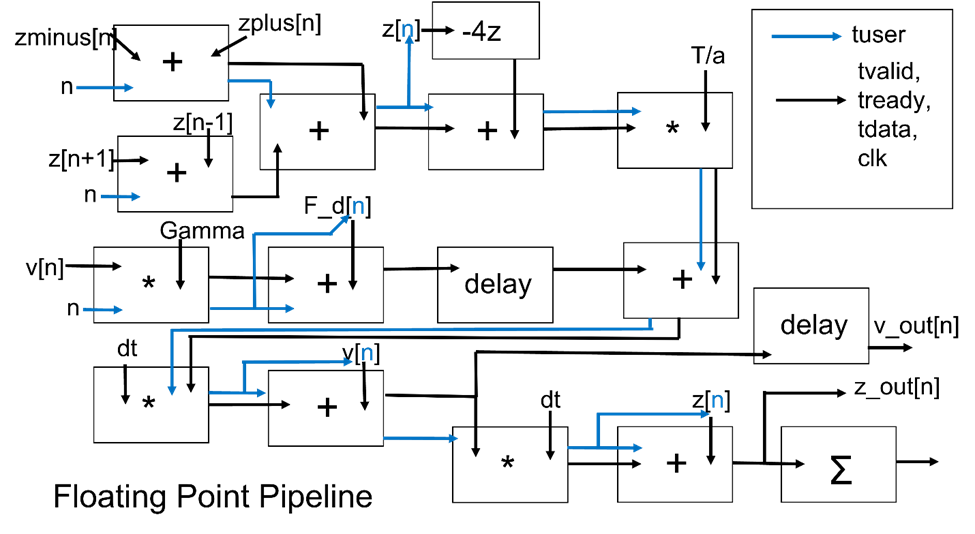
The basic idea was simply to convert each arithmetic operation in the force balance and Euler-Cromer method described above into floating point IPs connected to each other via AXI4-stream ports. This pipeline was meant to update the positions and velocities for a single column at a time. In the diagram, the z array represents the positions for the column being updated, and the zminus and zplus arrays represent the positions for its neighboring columns. The v array represents the velocities for the column being updated, and the F_d array represents any driving forces on the column you are updating. The driving forces were meant to be derived from a drum pad input, but for testing purposes, were controlled by buttons on the Nexys4 DDR board.

As you can see from the diagram, the operands for some floating point IPs are the outputs from other floating point IPs. That meant that if an IP had one operand coming from another IP and one operand coming from an input array, it would need to have some way of knowing which array index to use as an operand when an output is recieved from another IP. I accomplished that by streaming the array index through the pipeline with the TUSER signal. This allowed me to stream the inputs for a new mass into the pipeline every clock cycle.

In practice, the whole pipeline had about 50 clock cycles of latency. so updating the positions and velocities for each column took about 100 clock cycles not considering the latency associated with reading from BRAM. A burst of 50 sets of input values would go in, and 50 clock cycles later a burst of 50 sets of output values would come out. Not too bad overall.

There was also an IP at the end of the pipeline used to accumulate the sum of the positions for every mass in the system. This value was ultimately used to generate the audio signal.

The Results

The simulation with button inputs sounded pretty good. We only got a 25x50 mass system running at 20 ksps, but I was still pretty happy with it. I threw in some virtual IO IPs to adjust the position-sum-to-audio scaling factor, damping, and the tension (well, technically it was the tension divided by the grid spacing, which I called K). And once things were dialed in, it actually sounded like a drum!

I mapped different buttons on the nexys4 DDR board so that they would apply a driving force to different parts of the drum (e.g. the center or the edge), and the edge hits did indeed sound different than the center hits in the way I more or less expected. The main shortcoming was the distortion in the low amplitude parts of the waveform due to the 8 bit audio. As the amplitude drops off, the audio sounds more and more like a square wave due to the limited resolution, but that’s all we could get working given the dev board and time frame we were working with. See the video below.

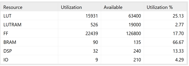
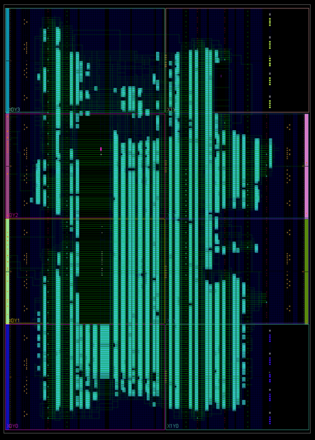
The design used up a lot of the Artix7’s resources, and routed signals all over the die! I suspect if I revisited this project I could not only vastly optimize the resource utilization, but also improve the audio quality by using a higher resolution external DAC or audio processor of some sort, but I haven’t had the time or urge to do that yet. One day though.

You also probably noticed that even though I described this as a drum pad, I didn’t mention the drum pad at all. That’s because my partner was the one working on that part of the project. He was using a piezo disk underneath a resistive touch screen to readout the force and position of a drum hit. He had his part of the project working at the same time as me, but we didn’t get to integrating the two until the day before the final presentation. That’s when I learned that they call it “integration hell” for a reason.

It should have been simple to take the force value read from the piezo and apply a proportional driving force to a mass in the simulation that corresponded to the position of the hit read from the resistive touch screen, but there was a number of scaling and fixed-to-floating point modules that had to go between those inputs and the simulation. It turns out that the few hours before a presentation really is not the time to figure all that out. Our builds suddenly hung for a long time in place and route, and, while they did complete, it was clear from the sound of the audio that something wasn’t right. We reverted our design to an earlier version, gave the presentation primarily using button inputs, and never revisited the project.

That is until I opened up the vivado project about a year ago and realized there was an egregious timing violation in our design. I wasn’t very privy to timing reports back in school, but a little professional experience goes a long way. I still haven’t tracked down what causing it because I don’t have the drum pad hardware or dev board to do any testing or debug. I simply removed the logic that inserted driving forces from the drum pad, leaving only the force inputs from the button. The build completed with some negative slack time to spare, so that’s what made it into the github repo linked above.

One day I hope to revisit this project and get it really dialed in, but without a percussionist to work with and draw inspiration from, I’ve moved on to other projects and interests for now.